Part II – Effect of High School on Final Board Examination –The Analytical Treatise
Dr. Shree Nanguneri and Co-Author-Project Lead Contributor, Ms. Reethika S. Iyer*
Background:
In Part I, we shared our experience on how parents make decisions to selecting high schools. Once the students graduate they are then again faced with the dilemma on what college or university they need to attend.
Value Proposition:
While looking at the investment in a child’s high school education it could run at an average of Rs. 35,000 per child per year. This translates to about USD 700-800 per child per year. This may look like peanuts to parents in the west, however this investment constitutes about 50 % of the salary of middle class families and about 20 % of the disposable income for the poor getting their children educated.
The recent survey states…..
” The 2,000 working parents across were surveyed across nine cities — Delhi, Mumbai, Lucknow, Dehradun, Pune, Bangalore, Kolkata, Chennai and Chandigarh—during April and May this year. One in 10 respondents said the cost of schooling did affect the choice of school. These were parents of young enough kids who had the option of changing schools. 65 % respondents said more than 50 % of their salary was spent on their children’s education while 50 % conceded schooling was actually a ‘strain’ on the family budget.
Nearly 60 % of parents felt education had become a business and that the high tuition fees did not actually indicate the academic standards of a school. Rather, it indicated a demand-supply function so that school managements could affect erratic fee hikes every year—something parents cannot protest. Even private preparatory schools charge Rs. 25,000 a term, the survey says.”
The key finding in this study which is in line with our hypothesis was “high tuition did not actually indicate the academic standards of a school.” So in our value proposition as indicated by the business value in the project charter of Part I, we will show how parents can take a decision based on facts regarding the following:
- Is the commute to a school further from home worth it?
- Will the additional tuition really paying off for their child?
- Are there significant long term benefits in the entire school selection process?
- How do we define a decision criterion for the selection of high school?
In this treatise on graphical and statistical analysis, we will present one isolated finding over a two year period on the same schools with no significant change either in the examination curriculum or student demographics.
Scope of Study:
- What is included in this study?
- High School as a variable
- Student count (minor variation)
- Year of Board Examination (2009-2011)
- Subject or Course of interest (core courses are constant)
- Includes analysis by subject and by aggregate score
- What is excluded in this study?
- General curriculum covered by school (CBSE standard)
- School’s extracurricular activity
- School’s after-coaching program
- Student’s after-school coaching program
- Performance of incoming students into their final year at school
- Support system offered by parents and family members at home
- Financial ability of parents
- Students residential area in metropolitan
- Root causes of why a school is better than the other
- Unexpected marginal error on data downloaded from the CBSE website
In this Part, we will share our analytical conclusions from our pilot study over the years 2009-2010. Our co-author has also graduated from one of the area schools chosen and is very much familiar with the systems and structure provided as part of the school infrastructure.
Data Structure:
Data has been downloaded as shown on the logbook available each year from the resource and format indicated in Part I of this series. Each student candidate has a score for the subjects they have taken and the associated absolute score achieved as reflected by a percentage in marks. An equivalent grade point average is also ascribed against the score based on a pre-determined cut off limit. From a value proposition point of view, our co-author and project intern has also researched and developed the following data for the corresponding schools in our analysis:
- Annual investment in tuition paid per child
- Commute distance per day between residence and school
- Commute time per day between residence and school
Analysis and Conclusions:
Our lead project contributor has followed the LSS DMAIC strategy in her problem solving methodology.
All analyses presented here is a sample given the brevity of this blog whereas the detailed report will be available later this summer when we publish this in a scientific journal of choice.
The basis of her analysis is supported by the GAP approach which constitutes:
- Graphical Illustration for visual analysis
- Analytical interpretation in our statistical treatise and a
- Practical interpretation as to what it means for this audience
Our analysis in the last section of this article is deliberately kept simple and short without going into too much statistical detail. The purpose is to enlighten our readers (who have all attended some form of school and/or college and can comprehend the barriers to making decisions in their day-to-day lives. This becomes all the more serious when they are related to the future of their children or someone close to them in their family, friends or peer network.
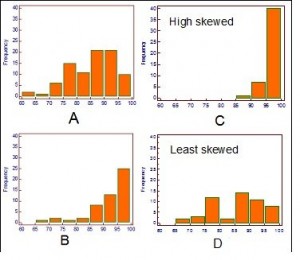
Figure 1: Histogram of Scores on an Individual Subject “Computer Science”
There is a general observation that students at School C were skewed toward higher computer science scores than any other school.
Figure 2: Box Plot Showing Scores on Individual Subject Computer Science
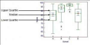 Students of School C showed the least variation and highest median for computer science scores.
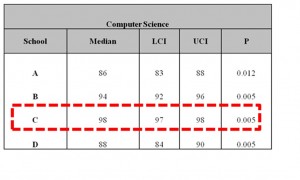
Table 1: Median Scores of Students in Computer Science at all Schools
The statistical table above indicates that Students’ scores at School C were statistically different from the rest of the schools as seen by the lower confidence (LCI) and upper confidence interval (UCI) values.
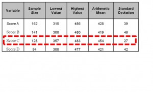
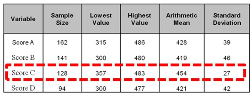
Table 2: Statistics of all Students at all Schools for their Aggregate Scores
The table above indicates that although Students’ aggregate scores at School C were statistically unique in their highest mean, there were students from other schools who also fell within the same range as School C. This tells us that School choice alone doesn’t necessarily mean a higher score for the individual student. One has to understand what is beneath the level of school and student that makes this possible. It does point out that the variation in aggregate scores were the least for School C leading us to believe that they post a higher consistency among their students.
Figure 3: Box Plot of Aggregate Scores of all Students from all Schools
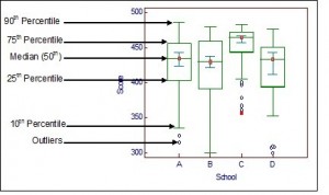 This is also illustrated in the box plot for the aggregate score of all Schools where the median for School C is uniquely different from the 3 other Schools.
Table 3: Statistical Analysis using Kruskal Wallis for Aggregate Scores in all Schools
The statistical table from above shows that “School C” is mutually exclusive from all the three other schools for the aggregate scores of all subjects put together.
Table 4: Overall Statistical Summary for all Subject Scores in all Schools
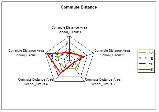
Figure 4: Spider Chart of Commute Distance for all Schools
This spider chart shows that the commute distance is the longest for School D.
Figure 5: Spider Chart of Commute Distance for all Schools
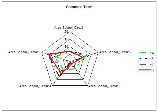 The commute time to school and back is varying by the region and school location.
Table 5: Probability of 25th Percentile to Qualify for Admission to any Program
Table 6: Probability of 25th Percentile to Qualify for admission to the ECE Program
 Tables 5 and 6 above, show an estimate of the probability of the 25th percentile qualifying for the minimum cut off as stipulated by a local university for its most popular engineering program.
While all schools display a low probability, School C does stand out uniquely and poses the highest probability of a student gaining admission into this engineering program. The lower table estimates the probability of any student from the school making it into the most popular program (Electronics and Electrical Communications). It shows that while all other schools are teetering below 1 %, School C has an 8 % probability for a successful admission.
Figure 6: Spider Chart on Tuition fees (INR) for all Schools
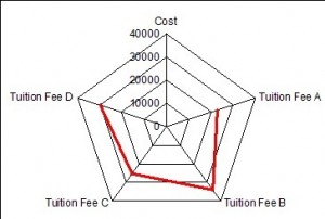 This spider chart tells us although School C came out as a unique environment to seek the highest probability and median score, it was associated with the least in tuition fees. This also agrees with the national survey on how higher tuition didn’t necessarily reflect a better academic performance of the students in a particular school.
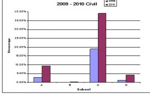
Figure 7: Probability of Admission into the CE Program for years 2009 and 2010
This bar graph compares the shift in probability of qualifying shift for a specific program (Civil Engineering – CE) for the students at different schools. The probability seems to have increased for Schools A, C, and D (School B is not even on the charts bearing a low probability for 2009 and 2010), while School C expectantly showing the highest increase as well as the highest among all schools.
In this article we have concluded that while the 4 Schools in our pilot study showed variation in student performance by subject as well as aggregate scores in their final examination there were some unexpected conclusions even in our limited scope of study:
- Students from the school scoring the highest didn’t pay the highest in tuition fees.
- Individuals from other schools scored higher than the median from School C.
- Commute distance or time didn’t have much to do with student performance.
- Probability of admission into a local engineering program can be measured.
- 2009-10 trends were similar for schools while ‘11 and ‘12 will also be evaluated.
We have an opportunity to investigate at the operational level of students to integrate a higher scope and truly understand the root causes of student success by mere final examination scores. Most parents in the east elect this as a decision criterion as it correlates well with the success of college admission in the eastern continents.
In Part III we will showcase the success of the project lead contributor on how she predicted her examination and mid-term test scores to decrease the time she devoted toward study time in a given semester of study at college. The student has more time in a day to engage in activity that is not academic in nature.
About the Authors
Ms. Reethika S. IyerI am a 3rd year undergraduate studies (B. Tech) student at SRM University, Chennai (India) majoring in the field of Information Technology (IT). One of my current key areas of research interests is “High School and Collegiate Student Performance Excellence” in India. This internship project aims at quantifying the relationship between the choice of high school in India and its impact on a student’s short and long term career. I have been fortunate to be mentored and coached by Dr. Shree Nanguneri, CEO, MGBS Inc. In this internship at MGBS, India, I have acquired a few critical Project Management and Planning (PMP) and Lean Six Sigma (LSS) problem solving skills which I have used in different areas (From planning for higher studies to predicting grades at college). In future I will be executing projects at higher level of complexity that will have a social significance at a global level which excites me professionally as well as provides an opportunity to significantly contribute to the society and make a difference. I plan to adapt to a professional career applying the skills of PMP, LSS, and IT while in parallel, pursuing my higher studies in the field of business administration. |
Dr. Shree NanguneriI am a business process improvement coach and consultant and have worked with several corporations in different continents over the last two decades. After having a successful 6-year work experience at GE, I started my own consulting company in 2000. I have been fortunate to successfully deliver across a variety of industries that include the fields of manufacturing, transactional as well as service type environments. I have published a few articles, authored patents and releasing a book in mid 2011. Although not an expert, I can converse reasonably well in Dutch, and Spanish, skills I acquired while working there. To date, the total annualized direct customer benefits from my services have accrued to several hundreds of millions of dollars. I enjoy outdoor activity, meeting people on a global level to mutually benefit each other. I am also thankful to my mentor as well as network members without which some of the achievement listed here would have been impossible. |

